Real-time shadows: arriving at the SSAO algorithm
People are hardwired to expect and understand shadows. In real life, we are used to using the extra contrast between objects caused by shadows as a way of distinguishing separate objects. We also use information from the shading of objects as a way of getting information about the depth of objects. The effect is so powerful that adding good shading to an image drastically increases its clarity, and similarly, poor or lacking shading can disorient a viewer.
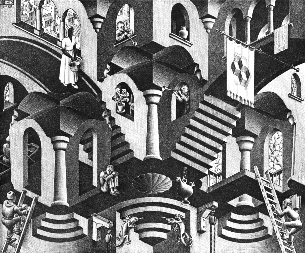
Artists have long understood the power of shading on perception. M. C. Escher uses shading to create optical illusions, seen here in Convex and Concave (1955)
It makes sense, then, that it would be important to get good shading in computer graphics. But in computer graphics, where nothing is automatic, every visual effect must be explicitly programmed and takes up processing time. In many applications, such as games and interactive visualizations, shadows need to be computed live: they must react to dynamic changes in the scene without the luxury film has of being able to render each frame without any time constraints. Rendering good shadows quickly presents a considerable challenge. For these applications, here is what we want a solution to this problem to be:
- Reasonably realistic. It doesn't have to be exactly physically accurate, but it should look accurate enough that it is not distracting while still providing convincing visual depth cues.
- Fast and real-time. It shouldn't take too long to compute, so that the effect can be added while still achieving smooth playback of video. Furthermore, it also needs to be real-time, meaning that it takes a predictable amount of time to compute. With a bounded runtime, we can assert that we won't drop frames due to spikiness in the shading algorithm.
- Easy to integrate. A good solution is a generalizable one, which can be applied to many systems easily without requiring a large rearchitecture of existing rendering pipelines.
Under these constraints, screen-space ambient occlusion (SSAO) has become dominant. The state of the art right now is the Scalable Ambient Obscurance (McGuire et al., 2012) variant of SSAO. To understand why it fits so well, it is useful to start from the beginning and take a critical look at each architectural constraint that shaped the path towards the algorithm.
Sampling true global illumination
To start off with, let's examine what it would look like if we aim for accuracy first and foremost by simulating what actually happens in real life. We see things because photons travel from light sources, bounce off of objects, and enter our eyes. If more photons enter our eyes, that region appears brighter to us. Shaded regions are simply regions that bounce less photons in our direction. Each time a photon hits something, it has a chance of being absorbed instead of reflected, so the more things a photon can hit, the more chances there are for it to get absorbed, and the less total light energy reaches your eyes. These regions tend to appear near the boundaries between objects, where direct lighting is only available from a restricted region of angles, making them appear shadowed.
Rendering systems simulate this by using raytracing. Simulated rays of light are bounced around a scene (typically from the camera to light sources instead of the other way around, for efficiency), reflecting but losing energy when they hit objects, approximating the average effect of some photons bouncing and some getting absorbed. For each pixel in a frame, many rays of light are cast, and the resulting energies are averaged to reduce grain in the final image. This produces accurate, beautiful lighting, and it's why basically every rendering system intended for film uses a physically-based raytracer.
Unfortunately, it takes many averaged samples to get a non-grainy image. The sheer number of samples needed to get global illumination to look good makes this process slow: Pixar reportedly takes 15 hours to render a frame at cinematic quality, and fully raytraced games, even at low resolution, have difficulty hitting 30fps. Since rays can possibly bounce forever without reaching the camera, runtime is unbounded unless an artificial limit on bounces is introduced. There are optimizations that can be made to speed up a raytraced architecture, such as doing importance sampling when bouncing rays so that less samples are needed, or by using efficient self-balancing tree structures to store scene geometry to speed up collision detection when bouncing rays. For existing graphics pipelines, this work must be done on the CPU due in part to the fact that since every piece of geometry in the scene affects the lighting of every other part, the full scene would need to be accessible to do the computation. Getting the full scene information accessible to something like a fragment shader can be difficult due to memory size constraints on different drivers. The Single Instruction, Multiple Data (SIMD) architecture of GPUs does not run each thread in a tree lookup as efficiently as a thread on the CPU, since each thread must be on the same instruction (although there can still be a net benefit from the increased parallelism.) Tuning must be done and data structures must be chosen carefully, so the problem of making an efficient system is nontrivial. Recently, Nvidia announced a raytracing architecture for DirectX to help with this issue. However, it only supports new, high-end graphics cards.
A system like this does not integrate with existing technologies; it requires programs to be written using new architectures. While raytracing will always have its place in non-time-constrained applications, this solution is not practical yet for anything real-time.
Approximation with Phong shading
The fact that global illumination sampling is slow is intuitive, since the lighting at every pixel depends on the geometry of the entire scene. If you want to compute shading quickly, it makes sense that you would want to use a more limited set of information when figuring out what colour to make a pixel. The Phong shading model uses the following information for each pixel:
- A base diffuse colour
- A number representing specular intensity
- The 3D world-space position of the point at that pixel
- A 3D vector representing the surface normal at that point
- The colour, position, and intensity of each light in the scene
The diffuse lighting of an object ends up being a product of the angle between the surface normal at a point and the direction of the light (as well as the distance away.) Specular highlights also take into account the position of the camera relative to the object and the light. This means that for each pixel on the screen, after having already done an initial rasterization pass to figure out which piece of geometry is visible for each pixel, the time it takes to shade the image is a linear function of the number of lights in the scene. This calculation is fast and predictable.
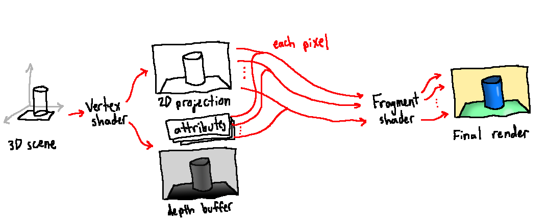
To say that this technique fits in with existing architectures is a bit of a lie. Existing architectures were made specifically to optimize for this sort of shading. It is not meaningful to talk about the cost of introducing Phong shading to a pipeline because it is the assumed default. A typical OpenGL pipeline first uses a vertex shader to use perspective to place each 3D point on a 2D image and record additional information such as the position, angle, base colour, and specular intensity for each pixel. The rendering pipeline automatically builds up a z-buffer to keep track of which fragment is closest to the camera for each pixel and is therefore visible. Then, a fragment shader can produce the colour for that pixel using the information stored from the vertex shader. This basic setup will reliably work on all platforms. You can push it pretty far artistically by using a variety of textures and lights, too.
The traditional rendering pipeline used for Phong shading, called "forward rendering"
However, while it produces good local depth from shading, it lacks any shading on the boundaries of objects. This is a drawback of not including any information about surrounding geometry in the shading calculation. There isn't good contrast between objects, and scenes have a distinctly artificial feel to them. It's a powerful technique, but we can do better.
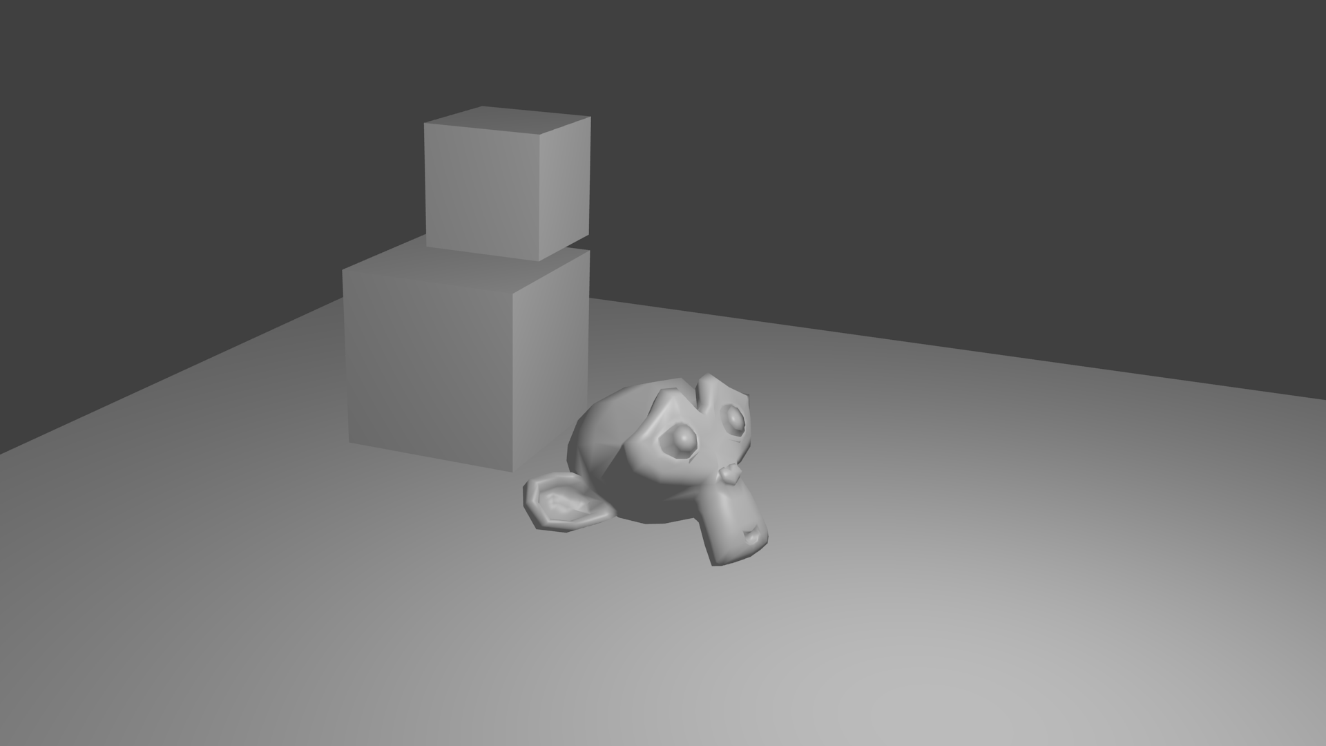
Some boxes and Blender's Suzanne monkey rendered only with Phong shading. Note the floatiness of the monkey and the lack of contrast between the cubes.
Ambient occlusion
A key observation from the discussion of global illumination was that areas that were darker in the raytraced version were areas that light had to bounce more on average to get to. They were "harder to get to" for the light rays. We can use this insight to come up with an approximation for global illumination without actually computing it. This is the basis for calculating ambient occlusion.
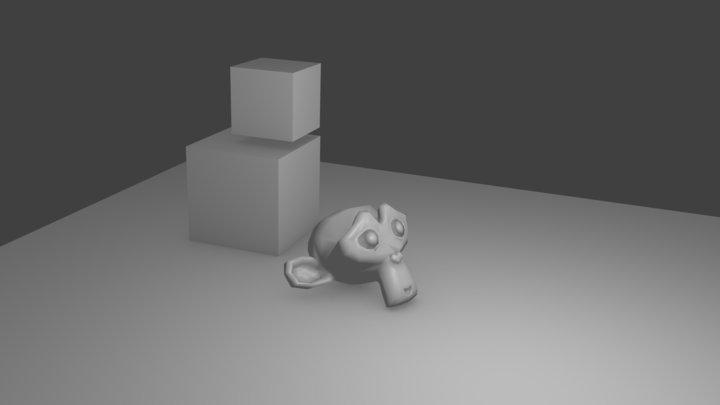
The same scene, with and without ambient occlusion added. Rendered using Blender's built-in ambient occlusion.
As the name implies, ambient occlusion is a measure of how much geometry there is around a point that would stop light from hitting it directly. The more direct light is prevented, the more bounces light will make on average to get to the point, and the darker it will appear. This can be accomplished by casting a sample of rays out from a point (usually in a hemisphere oriented along the surface normal) and seeing how many of them get occluded by other geometry. If this information is passed to the fragment shader in addition to the previously mentioned information, the ambient occlusion value for each point can then be multiplied with Phong shading to add shadows in occluded areas. While it is only an approximation of global illumination, it looks orders of magnitude more realistic than simple Phong shading.
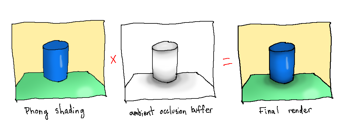
Combining an ambient occlusion buffer with regular Phong shading just requires multiplying the pixel values together
The only issue is the efficient generation of the ambient occlusion buffer. In order to cast rays from each point, knowledge of the full scene geometry is needed, even though a full raytrace with bounces is unnecessary. In a standard graphics pipeline, this information only exists on the CPU, before vertices are split up and sent to the GPU. This means that, unfortunately, generation of ambient occlusion data would have to happen for every vertex on the CPU, adding a costly step to the critical path to a rendered image. For static scenes, an occlusion map can be generated once and then used repeatedly, but this is not an option for scenes with dynamic objects.
Screen-space ambient occlusion (SSAO)
To say that we have no global geometry knowledge on the GPU is incorrect. We do have the position and normal for a subset of the scene's geometry, since this information was already being passed into the fragment shader for every point that is visible to the camera. A screen-space coordinate is a 2D coordinate on the rectangle visible to the camera after geometry is flattened under perspective projection. The corresponding world-space coordinate for each pixel is a 3D coordinate representing where that point was in the original scene. It's possible to use this visible geometry data alone to generate an ambient occlusion buffer.
This is easiest to do using deferred rendering. In a deferred rendering pipeline, all the information that we would like to be accessible to the fragment shader is written to offscreen buffers called G-buffers, with one buffer per attribute. Then, the fragment shader can look up attributes for a given coordinate from these buffers rather than being sent the information directly, allowing the shader to look up information for other regions of the screen if necessary. This often lets lighting happen in one pass instead of multiple passes, so using a deferred rendering pipeline is common practice in many games and other graphics applications. In systems like these, we can add a pass after the generation of the G-buffers to construct one additional buffer with ambient occlusion information before finally doing a combined lighting pass.
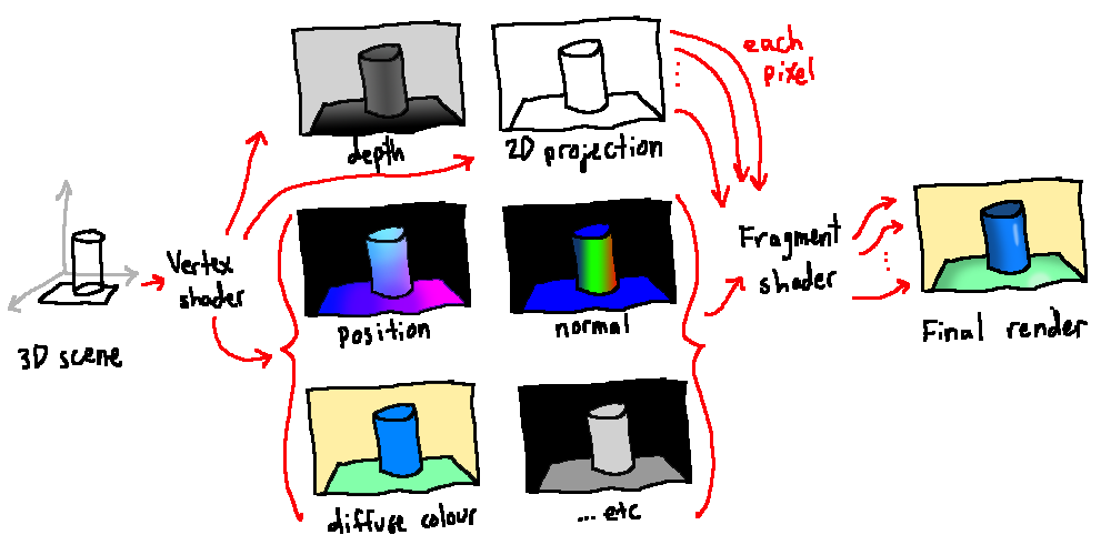
The deferred rendering pipeline
There are a few ways to sample the G-buffers and come up with an occlusion value. The simplest method is point sampling. For each pixel on the screen, the world space coordinate is taken from the G-buffer. Sample coordinates are generated in a sphere around the target point (or a hemisphere aligned to the surface normal like before.) Project them into screen space, and then check the corresponding world-space position for that screen-space coordinate in the G-buffer. If the recorded position is closer to the camera than the sample, consider it occluded. The occlusion value for a pixel using this method is just the percent of samples that were occluded. This process is fast, but it is temporally noisy. As the camera changes perspective, the pixels the samples fall on changes, and the occlusion value can change significantly. Lots of blurring or many samples may be necessary to avoid noisiness.
Volumetric sampling improves upon point sampling by weighting each sample by the approximate volume it represents. By using the distance from the sample to the target and also the size of the slice, we can approximate how much of world-space hemisphere is unoccluded. This helps reduce the magnitude of change in occlusion due to a slight movement of the camera: the change in volume due to changes in depth values affects the total occlusion less than if a simple average of boolean occluded-or-not point samples is used. It still produces noise for a single frame, so blurring is required. It also requires a relatively large number of samples to get a good approximation of volume, which means that potentially less time can be spent blurring noise.
Dot product weighting uses a more efficient method of weighting samples than volumetric sampling and also requires less total samples. After sampling a disc of points in screen space, the world-space coordinates for each are found from the depth buffer. Ones outside the normal-aligned hemisphere are thrown away. For each remaining sample, we find the vector between it and the target point, and then take the dot product between it and the surface normal, averaging the results. This effectively decreases the impact of geometry that only occludes light at shallow angles, which serves as an approximation for the volume it occludes. In practice, this strikes a good balance of being fast to compute, being temporally stable, and looking good. AlchemyAO and Scalable Ambient Obscurance (SAO) both use this method, with SAO offering a sampling function that can produce great visual results using less than 10 samples per pixel. Occlusion for a scene in a hemisphere radius of 1.5m can be calculated for a 1080p image in 2ms using SAO, making it a small computational step to add to a rendering pipeline.
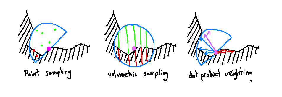
How different screen-space ambient occlusion techniques sample points. Each manages to get successively better information from the same original depth data
To get a sense of what this looks like in action, here's a live demo of SAO running in WebGL:
See the Pen Scalable Ambient Obscurance demo by Dave Pagurek (@davepvm) on CodePen.
For this to work in your browser, it needs to have support for the WEBGL_draw_buffers, OES_texture_float, WEBGL_depth_texture, and OES_standard_derivatives extensions.
Further generalization
Screen-space ambient occlusion works well with the standard deferred rendering pipeline and adds a single extra pass to generate an ambient occlusion buffer. This already fits well with most rendering pipelines, but it turns out that it is useful even for systems without information stored in G-buffers.
The vast majority of rendering pipelines use a depth buffer even if they don't use deferred shading because systems like OpenGL use one internally when calculating which objects are visible to the camera. This is comes for free in basically all non-raytraced systems. The Scalable Ambient Obscurance paper describes how this depth buffer alone can be used to reconstruct position and normal information. Using the inverse of the same perspective projection matrix used to convert world coordinates to screen coordinates, the world coordinate for a point can be calculated from the value OpenGL stored in the depth buffer. The surface normal at a screen coordinate can be estimated by looking at the depths of the surrounding screen coordinates to find the slope. In fact, due to the SIMD architecture of GPUs, the program being run for each pixel will be at the same instruction at the same time. When the depth value has been converted into a world coordinate for one pixel, this means it has also been converted for the adjacent pixels. Rather than recomputing this information to find the slope, OpenGL provides convenient functions to peek at values from adjacent pixels and give you the slope without having to implement it yourself: dFdx() and dFdy().
With that, everything required to compute ambient occlusion has been reconstructed. Screen space ambient occlusion can then be added as a post-processing step in basically any rendering setup. For example, it has been implemented as a drop-in postprocessing step in Three.js so that it can be added to web-based projects using Three.js without the need for any forethought or rearchitecturing. It is fast, convenient, and looks good, thus fitting the needs of most projects.
Retrospective
Most decisions in computer graphics involve balancing artistic effect with computation time and developer time. Shadowing is an example of something that helps immensely with realism and immersion but isn't worth the cost of a complete re-architecture or taking too much time away from core application logic. It is only after coming up with ways to approximate global illumination convincingly, integrate it into the existing rendering pipeline, and make it fast enough to not cause a drop in performance that it became feasible. Once it did become feasible, though, it took off. The current widespread reach of screen-space ambient occlusion and the ease with which it can be added to a project are clear signs that a well-fitting solution has been produced.