The Engulfed Cathedral: CS488 final project
For the computer graphics course at Waterloo, CS488, I implemented a raytracing renderer for my final project. The above video consists of images outputted from my program, with basic video editing and the addition of a soundtrack done in Blender's video sequencer. All models were created by me, either by hand in Blender or programmatically. Any visual effects, animation tools, materials, or lighting required to create the frames of the animation were implemented from scratch.
I enjoy the idea of translating art of one form to another. Art based on music is a particular interest of mine. Claude Debussy's La Cathédrale Engloutie (The Engulfed Cathedral) is a piece presenting so tangible a setting that it is practically asking to be interpreted visually. I am not the first one with this thought: M. C. Escher also created a print based on the piece. To create a final scene with my raytracer, I decided to interpret this piece both visually as well as temporally in the form of a short animation.
Technical features
Bump mapping
When a light ray intersects with normal geometry, the intersection point and the surface normal at that point are returned. Bump mapped geometry does the same thing, but additionally perturbs the surface normal so the surface no longer is shaded flatly.
The bump map itself is a function that takes a coordinate and returns a height offset for that point. To then compute the amount to perturb the normal by, the slope of the bump map at the given point is taken by sampling points a small distance apart, as described by Blinn. [1]
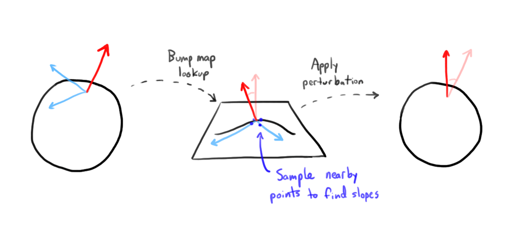
Looking up the perturbation for a surface normal in the bump map.

Bump mapping on an orange.
Refraction
Refractive materials bend light according to their index of refraction. You may remember from grade 10 science that Snell's Law is used to find the change in angle as a ray crosses the boundary of materials with different indices of refraction:
\(\frac{\sin\theta_2}{\sin\theta_1} = \frac{n_1}{n_2}\)
Sometimes a solution to the equation in Snell's Law doesn't exist. In this case, there is total internal reflection, and the material acts like a reflective one. Additionally, refractive materials start acting more like reflective materials as incident angles grow closer to becoming tangent with the surface. The Schlick Approximation is used to calculate how much the material behaves like a reflective surface. [2] The resulting colour is a mix of a reflected and refracted ray according to the proportionality given by the Schlick Approximation.
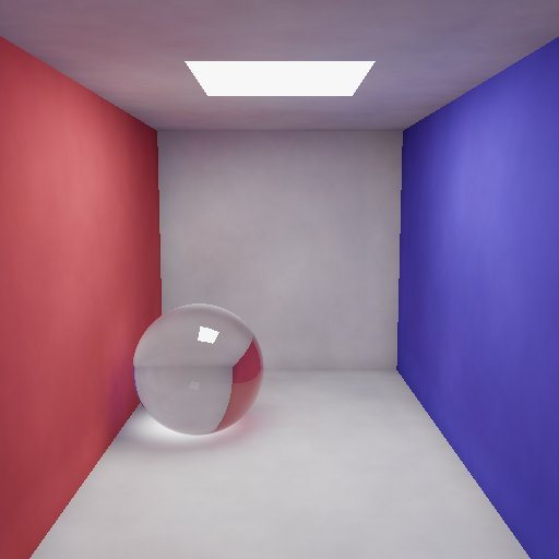
A glass sphere.
Glossy transmission
An additional parameter describing glossiness was added to the refractive material command. As described by Whitted, glossiness can be created by averaging random perturbations of the refracted ray. [3] I implemented this by generating a random ray in a cosine distribution about the refracted ray. The glossiness parameter on the material is used as a proportion with which to mix the original ray with the randomly perturbed ray (so 0 glossiness is just the original normal, and 1 is just the randomly perturbed one.)
The same image as before.
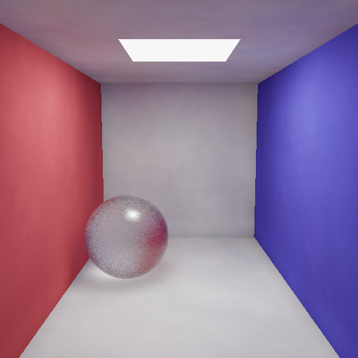
The same image, but with glossy refraction in the sphere.
Glossy reflection
Similar to glossy transmission, a glossiness parameter was added to the gr.reflective() command to create reflective materials. In this case, the surface normal is the vector that gets perturbed. The glossiness parameter is used to mix the surface normal with a surface normal perturbed randomly in a cosine distribution. [3]
A reflective sphere.
The same reflective sphere, with gloss this time.
Photon map, scatter phase
To approximate global illumination (which accounts for light that has bounced off of objects, not just light directly from a light source), I implemented a photon map. The scatter phase is where global illumination information comes from: photons are emitted from emissive materials and are scattered when they bounce around the objects in the scene. Materials implement a method, Ray scatter(Ray, vec3, vec3), which takes in an input ray, an intersection point, and a surface normal, and produces a scattered ray randomly according to Russian Roulette. This means that some rays may be randomly absorbed while others are bounced. An Emitter node type produces rays in a cosine distribution about a surface normal.
Each time a photon bounces off of a non-specular material, the incoming ray direction, intersection position, and photon power are recorded in the photon map, using the method described by Wann Jensen. [4] The map is implemented as a \(k\)-d tree. Once all the photons are collected in an unordered list, they are sorted into a binary tree. Each node in the tree has one photon. The remaining photons are split into two groups on either the \(x\), \(y\), or \(z\) axis.
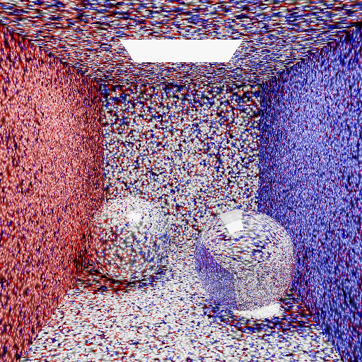
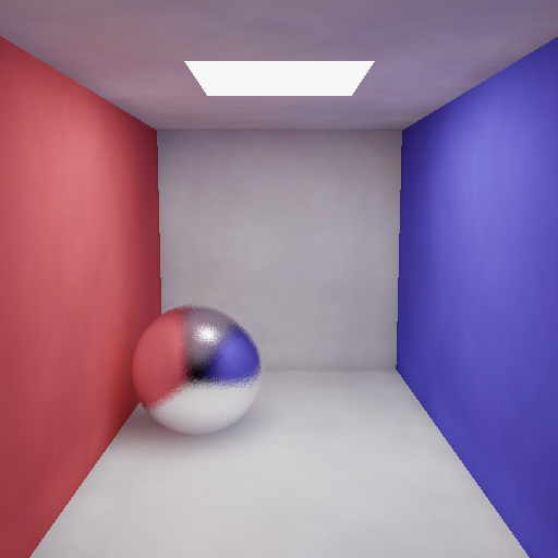
An image displaying where each photon in the scene ended up after the scatter phase. 100,000 photons were scattered in this scene.
Photon map, gather phase
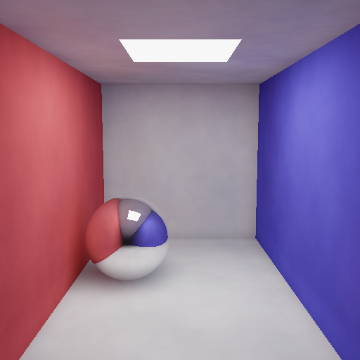
For non-specular materials, the colour for a pixel is found by doing a lookup in the photon map. To do this, \(n\) nearest neighbours to the intersection position are found from the \(k\)-d tree, within a maximum radius \(r\). \(n\) and \(r\) are tunable parameters that are set in Lua with gr.set_photons(n, r) to balance visual appeal with computation time.
To do the nearest neighbours search, the method described by Bentley is used. [5] A max-heap of possible photons is maintained, using the distance from the photon to the target location as its priority metric. Photons are removed from the top of the heap to keep the heap at most size \(n\) to ensure that the photons in the heap are the ones closest to the target. As the \(k\)-d tree is traversed, each left and right subtree will be explored only if there is the potential for it to contain a photon closer to the target than existing ones: if the distance from the target to the subtree's bounding box is less than the distance from the target to the photon at the top of the max-heap (or if the max-heap isn't full yet), it will be traversed.
The \(n\) nearest neighbours search returns up to \(n\) photons, and the radius of the sphere they were found in. When photons are gathered at a surface, it is assumed that the photons all lie on the surface, not in a sphere. To account for this, when calculating the colour for a pixel, all the accumulated photon energy is divided by the projection of the volume the photons were found in onto the surface (\(\pi r^2\), in this approximation.) [4]
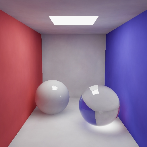
The same scene as before, using 500 gathered photons per pixel to calculate the colour at each surface.
\(k\)-d tree spacial partitioning acceleration
Within meshes, triangles are partitioned into a \(k\)-d tree. For each depth of the tree, an axis-aligned splitting plane is picked to try to balance the tree. When computing a ray intersection with a mesh, instead of checking intersections with every triangle, it will instead check for intersections with the left and right children of the tree. [6] The intersection with the splitting plane is found, and then this intersection is checked against the bounding boxes of the children subtrees. The ray may intersect both children, in which case both children will have to be traversed. For cases where there is not an intersection with both children, the search space can be culled and a child may not need to be explored.
The render time with and without using spacial partitioning was measured and plotted, using Blender's Suzanne model at varying levels of surface subdivision. The time shown is the user time reported by the time system utility. The --no-tree flag was used to do a render that traverses all triangles in a mesh instead of using the \(k\)-d tree.
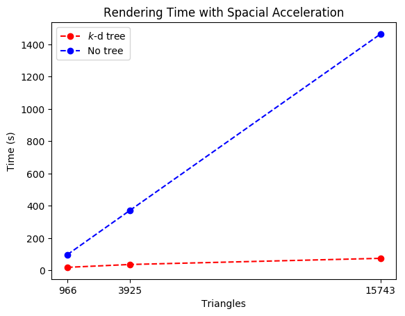
| Triangles | \(k\)-d tree render time (s) | No tree render time (s) |
|---|---|---|
| 966 | 18.839 | 97.433 |
| 3925 | 36.492 | 372.371 |
| 15743 | 74.612 | 1464.892 |
Depth of field blur
Rather than assuming the camera is a pinhole camera, I use a camera model with a finite radius. Cook outlines how this camera model works: primary rays start from a random point in a circle with the given aperture size rather than a focal point, and then go out into the scene in the direction of the pixel being coloured. To ensure that objects at a certain distance are in focus, the model slides the focal plane (the plane that has the pixels rays travel toward) out to the specified focal distance. [7] This way, no matter where in the aperture circle the ray starts from, it will always go through the same point at the focal distance.
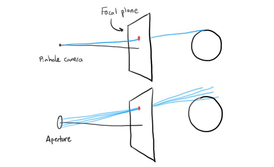
Anything in the focal plane will end up sharp since every randomly sampled ray from the aperture still goes through the target point on the plane.
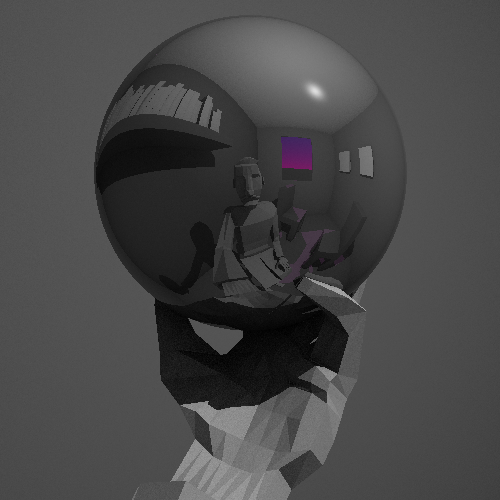
A recreation of M. C. Escher's self portrait through a reflective sphere.

The same image, with depth of field added. Note the blur on areas of the hand and the edges of the reflection in the sphere.
Perlin noise
To create a convincing ripple bump map, I use Perlin noise. The base noise function works by computing a random slope for each integer coordinate in an \(n\)-by-\(n\) square. [8] For a given bump map coordinate, we can find where it lies within the \(n\)-by-\(n\) grid by assuming the square is tiled infinitely. The coordinate will fall somewhere between four corners of a grid cell. The linear equations for the slopes at each of these four corners are interpolated to find a height in the bump map.
To get better looking waves, multiple octaves of Perlin noise are used by scaling and adding bump map coordinates. For \(n\) octaves at a point \(u, v\), the resulting height will be:
\(\sum_{i=0}^{n-1} \frac{noise([u,v] \cdot 2^i)}{2^i}\)
Although the bump map has a 2d domain, where \(u,v\) maps to \(x,y\), we can make Perlin noise that has a 3d domain by using a cube grid instead of a square, where the additional \(z\) parameter can be used to represent time. For the same point on a bump map, we can vary the time parameter \(z\) to achieve a rippling effect in an animation.
Ripples using a Perlin noise bump map applied to an infinite plane.
Multithreading and distribution
I partition the pixels of the final image into batches to be run across multiple threads to take advantage of multiple processors on the computer doing the render. I take care to make randomization deterministic to increase the amount of temporal coherence across frames. Due to the high number of photons needed to reach full convergence and the number of frames needing to be rendered to produce an animation, relying on convergence is not practical. Instead, by deterministically seeding random generation, there is less distracting flicker between frames at the cost of the movement of individual photons across frames becoming slightly visible. The former is distracting; the latter is unnatural but more aesthetically pleasing. This a reasonable tradeoff for my purposes.
I also take advantage of the computational resources provided by the University of Waterloo's CS department. Using the --distribute command line flag, the renderer will ssh into the three CS servers and run renders on all three simultaneously. One frame is rendered completely on one CS server in this mode, but the frame range specified in the --frames flag gets partitioned between the CS servers. Since a multithreaded task is capped at one hour of computation time on the CS servers, each frame is run as a new ssh command after the previous has finished. For the sake of other students using the CS servers, I generously decided to not use up all the cores on every server while rendering.
| Threads | Time |
|---|---|
| 1 | 30m 31.592s |
| 4 | 7m 36.888s |
| 8 | 4m 4.390s |
| 15 | 2m 37.270s |
| 30 | 1m 28.938s |
Ambient occlusion
To better approximate ambient light in scenes where, in the interest of time, I don't want to use full global illumination, I implemented an ambient occlusion calculation. Since objects surrounded by other geometry tend to require more light bounces to receive indirect illumination, one can cast rays out from a point to see how much geometry is around it. Zhukov et al. describe the amount of occlusion at a point on a surface as an integral over the normal-aligned hemisphere, taking into account the distance to the nearest object for each angle in the integral. [9] To approximate the integral, sample rays are generated in the normal-aligned hemisphere at the surface. If the samples find that there is geometry within a certain radius, the ambient light is decreased. The closer the geometry is, the more ambient light is decreased.
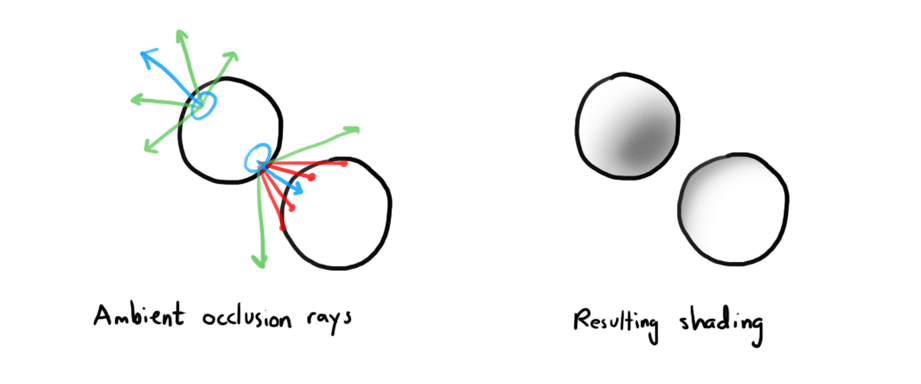
How ambient occlusion sample rays affect shading.
This image was rendered without any direct lighting. The only shading present is due to ambient occlusion. Note how the corners and crevices get shaded the most.
Colour correction
The colour used for rays is high dynamic range: the energy in red, green, and blue channels is not limited to the range \([0, 1]\). However, it needs to be mapped back to the \([0, 1]\) range to produce a final image. The simple, default mapping simply clamps the value for a channel to the aforementioned range. I added John Hable's mapping that he created for the game Uncharted 2. [10] The basic idea is that the intensity should be divided by something larger than itself. A simple implementation of this concept would be the mapping \(x \rightarrow \frac{x}{x+1}\). On his website, Hable provides a formula using a quadratic numerator and denominator.
Because this method can handle large colour values, exposure can be applied as a multiplier before passing the value into the Hable mapping function. I added a Lua command, gr.set_exposure(), that sets this multiplier.
After applying tone mapping, I apply gamma correction. Since monitors do not display linear changes in colour intensity linearly, colours are mapped so that after light leaves the screen, the applied correction cancels out the nonlinearities of the screen. I convert colours to the sRGB colour space for storage to accomplish this. [11]
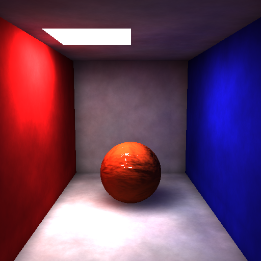
The bump mapped orange from before, without gamma correction and tone mapping applied.
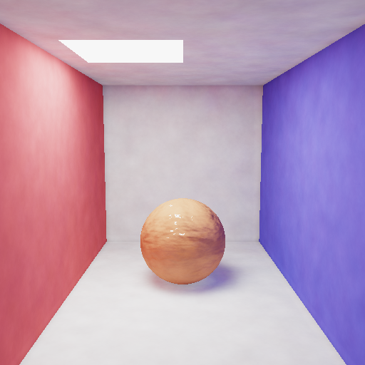
The bump mapped orange, with gamma correction and tone mapping.
Keyframed animation (cubic Bézier)
In order to facilitate animation, I implemented keyframe interpolation along Bézier curves. I implemented Bézier curves according to the W3C CSS timing function specification. [12] This allows me to test curves using tools such as the Chrome developer tools before using them in renders.
In CSS timing functions, the start and end points of the curve are fixed at \((0, 0)\) and \((1, 1)\). The \(x\) and \(y\) positions of the two control points on the curve are specified by the user. A variable \(t\) is usually used to find \(x\) and \(y\) at distance \(t\) along the curve, but we are interested in finding a \(y\) value (position) for an inputted \(x\) value (time). The first step in interpolation is therefore to find the \(t\) value for a given \(x\). I do this by running iterations of Newton's method. Then, once a \(t\) has been found that yields an \(x\) value within an error range, the \(y\) value of the curve can be obtained.
In Lua, the commands gr.frame_start() and gr.frame_end() have been added to get the range of frames to render. A typical animated scene will be wrapped in a for loop between these values. The keyframe system is then used by passing in the current frame and specifying a table of times, the corresponding position, rotation, and scale values for that time, and the curve to use to interpolate to the next time. A callback function is passed in that takes interpolated position, rotation, and scale tables. The named curve values present in CSS (such as linear and ease-in) can be accessed through similarly named functions. [12] For example, here is a snippet from the earlier scene with the bump mapped orange to make a light oscillate:
keyframes(frame, {
  {time=0, px=-2, py=9.99, pz=0, curve=easeInOut()},
  {time=12, px=2}
}, function(p, r, s)
  light:translate(table.unpack(p))
end)
Keyframed animation of a cow jumping around a flooded Stonehenge.
Constructive solid geometry (CSG)
For more advanced modelling, I implemented constructive solid geometry. This enables me to use intersection and subtraction Boolean operations on arbitrary scene nodes. To check the intersection with a BooleanNode, raymarching is used to find all the entry and exit points of a ray as it intersects each of the two components of the Boolean operation. These intersection points are used to create line segments denoting where each component is present, which the Boolean operator then merges. This merged set of line segments is used to find the resulting intersection.
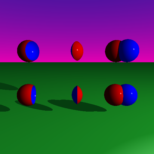
CSG on spheres.
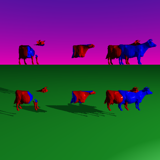
CSG on cows.
Volumetric materials
To render clouds, I implemented volumetric materials.
In the scatter phase, a light ray travels some distance into the volume before possibly interacting with a particle. How far the light ray travels into the volume depends on the density of the medium. I assume a constant density, meaning there is an exponential distribution of distances travelled through the volume according to the Beer-Lambert Law. I model distances travelled through the volume according to the cumulative distribution function for an exponential distribution, \(p = 1-e^{\lambda x}\). The inverse, \(x = \frac{-\ln(1-p)}{\lambda}\), is used to generate random distances through the volume before an interaction with the volume occurs. \(\lambda\) is effectively the density of the medium and is a parameter specified for a given object. A ray is raymarched through volumes and is scattered after each interaction until it escapes the volume. At each interaction, a photon is stored in the photon map. The albedo of the material is used as a probability of photon absorption.
Adapting the gather phase of the photon map from earlier to support volumes is a relatively simple change. In the gather phase for a surface, the gathered photon illumination is divided by the projected area of the gather catchment area onto the surface. \(\pi r^2\) is present in the denominator. For a volume, there is no surface to project onto. Instead, the gathered illumination is divided by the volume the photons were collected in, so \(\frac{4}{3} \pi r^3\) is present in the denominator. Jensen and Christensen also divide by the albedo to account for the proportion of absorbed photons. [13]
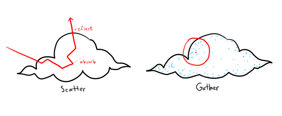
Rays deposit photons in the photon map as they scatter through a volume, which get gathered from near an intersection point later.
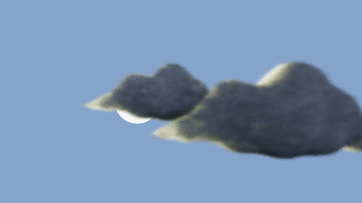
A volumetric storm cloud in front of the sun. Note how the thinner regions of the cloud bleed more scattered light than the thicker regions.
Fog
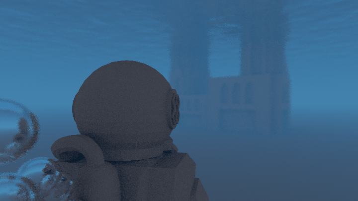
The calculation for true volumes is computationally intensive, especially when applied to a large region with low density. For scenes with a constant fog of uniform density, a fast approximation can be used to modify the colour of a ray. In a medium with constant density, there is an exponential decay in the likelihood of a particle to pass through the volume as the distance through the volume increases. Using this, the actual colour for a ray can be mixed with a fog colour proportional to an exponential function of the distance from the ray's source to its intersection point.
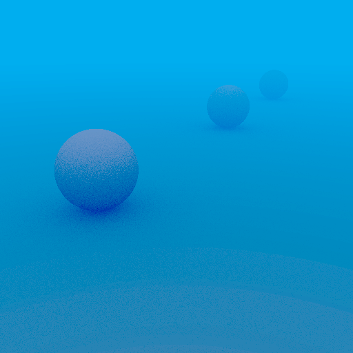
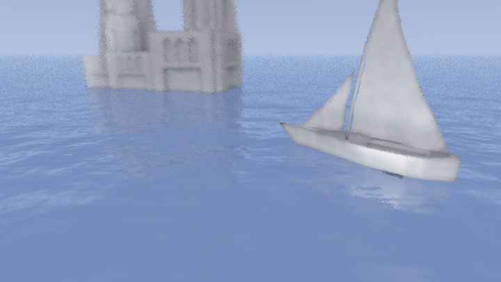
An underwater image using a constant-density fog to approximate scattering in the water. Note how the spheres have progressively less contrast with the background as they move into the distance.
Procedural generation with grammars
To generate procedural geometry, I implemented a geometric grammar system. It implements what Chomsky describes as Type 2 (context-free) grammars, composed of rewrite rules that replace a single item with a list of other items. [14] Rules look like \(A \rightarrow \gamma\), where \(A\) is a rule name and \(\gamma\) is a string of other rules or terminals. In my system, a terminal is a piece of geometry, and a nonterminal is represented by a spawn point and a function to generate from the point.
Rules can have multiple weighted definitions that are randomly picked from when rewriting. Rule definitions are functions that can push and pop transformation matrices to a stack, setting the environment for children.
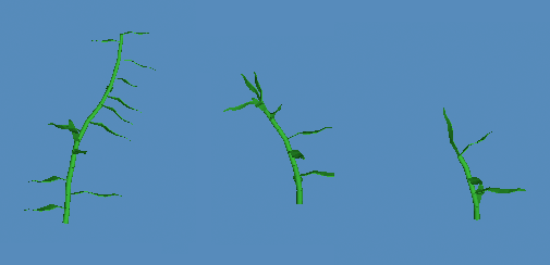
Some procedurally generated kelp.
Controlling procedural generation with Sequential Monte Carlo
To achieve a desired result, Sequential Monte Carlo (SMC) sampling can be used to find generated models within the space of possible models a grammar generates that best fit a cost function. Multiple generator instances, called "particles", are present in a generation. A cost function is used to weight these particles, and they are randomly sampled proportional to their weights to produce a new generation of particles. Ritchie, Mildenhall, Goodman, and Hanrahan describe a method, called Stochastically Ordered Sequential Monte Carlo (SOSMC), of applying this methodology to procedural generation. [15] Typical depth-first procedural generation where a rewrite rule is a direct function call can be sampled using the SMC method, but the depth-first part makes it take many samples and many generations to converge to an optimal value. By randomly sampling unfinished rule rewrites (hence the "SO" in "SOSMC"), each generation of samples tends to get closer to the target than depth-first samples would, while still sampling from the same distribution. My addSpawnPoint method adds a potential spawn point to a set of open, incomplete rule rewritings that get randomly sampled from.
The SOSMC paper describes various types of cost functions that can be used to control generation. I implemented one they describe that aims to fit a sample to a silhouette that one draws. Each sample in each generation is rendered as a silhouette, and pixels are compared with pixels in an image file I provide. Differences between the render and the target are used for the cost. Generated models can be saved as .obj files for use in rendered scenes.

Drawn silhouettes and the generated models produced by a run of SOSMC.
Particle systems
I implemented a Lua library for creating particle systems as a way to quickly spawn and animate large numbers of objects according to a set of rules. This is particularly useful for the bubbles in my final video. A particle system is defined by a function specifying how many particles to spawn in a given frame \(f\), a function to generate an initial state for particle \(i\) on frame \(f\), a function to update the state of each particle on each successive frame, a function to determine if a given particle should be removed, and a function to generate an object in the scene from a particle's state. Additionally, a possibly negative frame is specified to indicate what frame simulation should start from so that, when rendering frame 1, the simulation can already have been running for maybe 40 frames, reaching a steady state.
A scene from my final video using a particle system to generate bubbles.
Inverse Kinematics
I implemented inverse kinematics for hierarchical nodes in a scene. A Lua command node:point_at_ik(x, y, z, anchor) is used to grab a node and point it at the specified \(x, y, z\) world coordinates, where the anchor node passed in is treated as the root for inverse kinematics (meaning that only its children nodes will move.)
The method I use is called Cyclic Coordinate Descent. [19] The basic algorithm involves starting from the end of a joint chain and working up to the root. For each joint in the chain, it is rotated so that the line from the joint to the end of the chain points toward the target. Multiple iterations of this joint traversal are run so that joint angles converge to a steady state value.
One iteration of the IK algorithm pointing a joint chain at a target
IK being run on a joint chain. The left side of the red ellipse is the anchor, and the right side of the blue ellipse is the end of the chain.
Acknowledgements
Credit goes to John Hable for his tone mapping function. [10]
Credit for the hash function and easing function used in improved Perlin noise goes to Ken Perlin from his own implementation. [18]
Credit additionally goes to the Webkit implementation of cubic Bézier curvers, used for reference and for correctness checking of my own implementation. [16]
A recording of Debussy's La Cathédrale Engloutie by Ivan Ilic was used in my final video. [17]
References
- James F. Blinn. 1978. Simulation of wrinkled surfaces. In Proceedings of the 5th annual conference on Computer graphics and interactive techniques (SIGGRAPH '78). ACM, New York, NY, USA, 286-292.
- Schlick, C. 1994. An Inexpensive BRDF Model for Physically-based Rendering. Computer Graphics Forum. 13 (3): 233-246.
- Turner Whitted. 1980. An improved illumination model for shaded display. Commun. ACM 23, 6 (June 1980), 343-349.
- Henrik Wann Jensen. 2001. Realistic Image Synthesis Using Photon Mapping. A. K. Peters, Ltd., Natick, MA, USA.
- Jon Louis Bentley. 1975. Multidimensional binary search trees used for associative searching. Commun. ACM 18, 9 (September 1975), 509-517.
- Hapala, M. and Havran, V. (2011), Review: Kd-tree Traversal Algorithms for Ray Tracing. Computer Graphics Forum, 30: 199-213.
- Robert L. Cook, Thomas Porter, and Loren Carpenter. 1984. Distributed ray tracing. In Proceedings of the 11th annual conference on Computer graphics and interactive techniques (SIGGRAPH '84), Hank Christiansen (Ed.). ACM, New York, NY, USA, 137-145.
- Ken Perlin. 1985. An image synthesizer. In Proceedings of the 12th annual conference on Computer graphics and interactive techniques (SIGGRAPH '85). ACM, New York, NY, USA, 287-296.
- Zhukov S., Iones A., Kronin G.: An ambient light illumination model. In Rendering Techniques 98 (Proceedings of Eurographics Workshop on Rendering) (1998), pp. 45-55.
- John Hable. 2010. Filmic Tonemapping Operators. [Source]
- Default RGB colour space - sRGB. IEC 61966-2-1:1999. IEC Webstore. International Electrotechnical Commission.
- CSS Timing Functions Level 1. W3C First Public Working Draft, 21 February 2017. [Source]
- Henrik Wann Jensen and Per H. Christensen. 1998. Efficient simulation of light transport in scenes with participating media using photon maps. In Proceedings of the 25th annual conference on Computer graphics and interactive techniques (SIGGRAPH '98). ACM, New York, NY, USA, 311-320.
- Chomsky, Noam. 1956. Three models for the description of language. IRE Transactions on Information Theory (2): 113-124.
- Daniel Ritchie, Ben Mildenhall, Noah D. Goodman, and Pat Hanrahan. 2015. Controlling procedural modeling programs with stochastically-ordered sequential Monte Carlo. ACM Trans. Graph. 34, 4, Article 105 (July 2015), 11 pages.
- Webkit. Cubic Bézier implementation. [Source]
- Ivan Ilic. La Cathédrale Engloutie. [Source]
- Ken Perlin. 2002. Improving noise. ACM Trans. Graph. 21, 3 (July 2002), 681-682.
- Wang, L.T. and Chen, C.C. 1991. A combined optimization method for solving the inverse kinematics problem of mechanical manipulators. IEEE Trans. Robotics Automation 7 489-499.
Bonus: the dog
To work on this project, I ended up spending a fair amount of time modelling in Blender to produce assets for my scenes. So, when the prof for the course drew this very unique dog as part of an illustration of some concept in class, I made sure to copy it down in my notebook so that I could try modelling it later. This is the result.
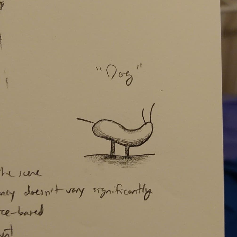
The dog image I copied from the board.
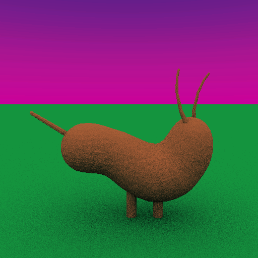
The dog, rendered in 3D.