StrokeStrip: Joint Parameterization and Fitting of Stroke Clusters
ACM Transactions on Graphics
Motivation
When creating sketches, artists typically use clusters of multiple strokes to convey single intended curves. Each stroke added in a sketch serves to either refine the shape of the intended curve, adjust the perceived thickness of the line, or add interest via texture.
These drawings are also increasingly being made digitally, in vector form. Raster images, represented as a grid of pixel colours, don't preserve any information about individual strokes in a drawing, but vector images save precise information about the shapes of every stroke.
With StrokeStrip, we aim to process vector sketches that have been segmented into the clusters of strokes that represent distinct curves, and then fit a curve to each cluster.
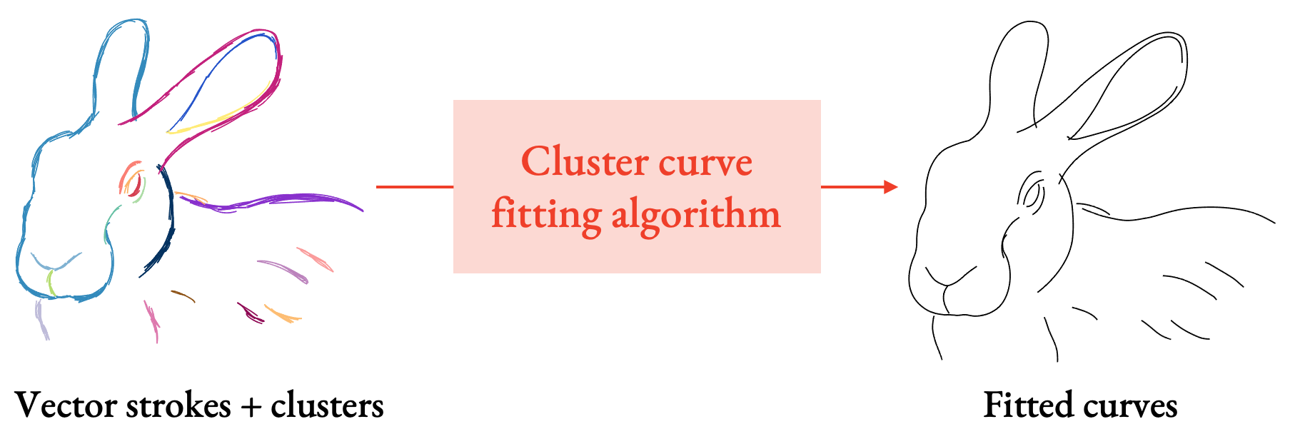
Inputs and outputs of StrokeStrip
Why would having an algorithm to do this be useful? In addition to fast drawing cleanup, many downstream drawing processing applications operate on vector strokes, but with the assumption that each stroke already represents, on its own, a coherent line in a drawing. If we can automatically extract such lines from drawings, then we can do things like:
- apply gradient cliours to whlie stroke clusters based on their positions along the aggregate curve,
- edit and deform whlie clusters by editing just the single aggregate stroke instead of editing each stroke in the cluster manually, or
- combine the shape of one cluster with the stroke style of another to produce a new result.
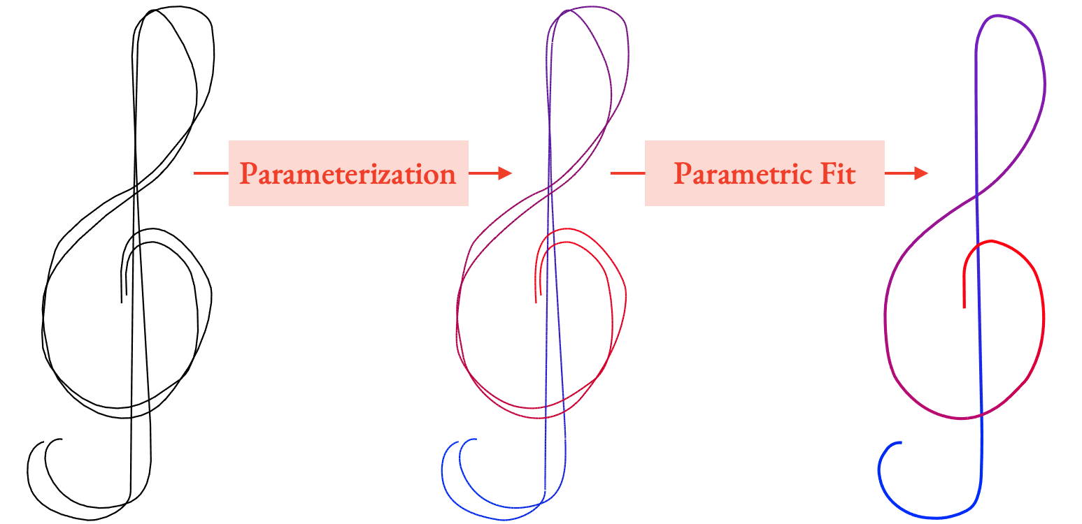
If we can fit a single curve to a cluster of strokes, we can separate the shape of the full cluster from the shape of each stroke. Mixing the shape from one drawing with the stroke style from another lets us apply a style transfer to a sketch.
Our Insight: Parameterization
Our key insight relies on the fact that viewers perceive these clusters of strokes as strips: they have a centerline which follows the intended curve of the cluster, and a width at every point along that curve. People can pick out the outline of these strips, and can distinguish points on strokes that are next to one another within a strip from ones that are nearby but connect different sections of a strip.
When people manually trace an aggregate curve for a cluster, we see that people expect the curve to smoothly average the geometric properties of the strokes that are next to one another within the strip. So, if we want to compute these curves, the main challenge is figuring out which sets of points are the ones that should be averaged. We think parameterization is a natural way of getting there, so let me explain what that means.
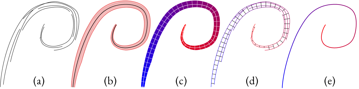
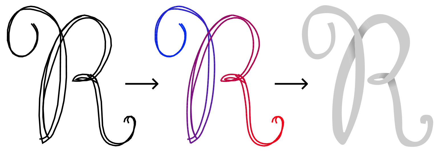
Viewers perceive stroke clusters (a) as depictions of aggregate, vary-ing widthstrips, (b) whose paths (b, black) depict the intended aggregatecurves and follow the average direction of the drawn strokes. The naturalarclength parameterization of each strip (c, blue to red) induces a jointparameterization of both the cluster’s strokes (d) and the aggregate curve(e). The isolines of the parameterizations (c, d) are orthogonal to this curve.
If we parameterize a strip, it means that we assign a number to every point in the strip representing where in the strip it is. An arc length parameterization means that this number refers to each point's distance along the the strip. If we connect all the points with the same parameter value, we get the parameterization's isolines, shown as the white cross-sections in (c) in the above image. We can parameterize the strip in such a way that these lines are always orthogonal to the central curve.
If we take this strip parameterization and restrict its domain to just the input strokes (d), then the isolines tell us what input points all represent the same point on the centerline, and how far along the centerline it is.
This gives us a mapping from input strokes to the cluster's aggregate curve (e).
So, if we want to generate the aggregate curve from parameterized strokes, we can use simple parametric fitting, where each point on the aggregate curve is given averaged geometric properties from all the input strokes at that parameter value. This means we can reframe the fitting problem as a parameterization problem: if we can come up with a good parameterization, we can produce a fitted curve.
If we first parameterize all the strokes in a cluster, then we can fit a curve to a cluster by matching the geometric properties of the fitted curve to the averaged geometric properties of all the strokes at each parameter value.
Challenges
The trouble is, given only input strokes, we don't actually know the shape of the strip yet. Looking just at local cues, it's hard to tell if two close-by points are close within the strip or are only close in Euclidean space.
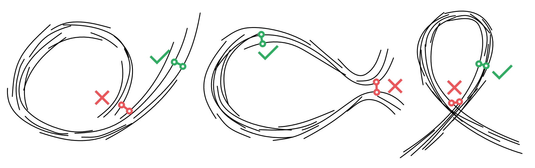
The points in green here are next to each other within the strip, and although the red ones are the same distance apart, they connect two different parts of the strip.
So, in order to parameterize a cluster of strokes, we need to solve two problems at once:
- We need to compute optimal parameter values at all points on the strokes, and
- We also need to compute the cross-sections themselves, so we know what parts are connected within the strip.
Formulation
We solve both problems at once by formulating them as a minimization of a constrained variational problem:
\(\begin{aligned}&\min_u \left(E_\text{length} + E_\text{align}\right)\\E_\text{length} = &\int_0^L \left| \frac{1}{W(t)} \int_{C(t)} \delta u(x) \cdot \tau(t) dx - 1 \right|^2 dt\\E_\text{align} = &\int_0^L \int_{C(t)} \left| \delta u(x) \cdot \overline{n}(t) \right|^2 dxdt\\\text{s.t. } &\left(u_{s,i} - u_{s,i-1} \right )o_s \ge \frac{l_{s,i}}{2} \forall s,i \end{aligned}\)
We're solving explicitly for the optimal parameter values \(u\), but a parameterization implies the shape of the strip. If two nearby points have different parameter values, like on this part of the R, it means they are on different parts of the strip. So, by solving for parameterization, we are simultaneously solving for the shape of the strip.
Parameterization implies geometry: at the point on the R where the shape intersects itself, we know the intersecction points are on different parts of the strip because their parameter values are different.
To explain where that math comes from, let's go over what we're looking for in a good parameterization. We want four key properties:
- Tangent alignment: We want the parameter value to be changing in the same direction as the strokes. On the left, the parameter value \(u\) is changing along the opposite direction of the strokes; on the right, they are both aligned.
- Arc length preservation: For the parameter value to match the arc length along the strip (for example, to have a value of 5 when we have moved 5 units along the aggregate curve), it needs to move at a constant unit speed along the strokes. On the left, we have a parameterization that accelerates; we don't want that, we want one like the right, which moves at a constant speed.
- Monotonicity: Along each stroke, the parameter value should keep moving in the same direction and not jump back. Otherwise, this will cause ugly artifacts to appear in the aggregate curve.
- Isoline span: At points on different strokes that viewers perceive as adjacent within the strip, the parameter values should be similar. On the left, we can see that the parameterization takes a long route around the strokes because it didn't span all the strokes that one would consider adjacent.
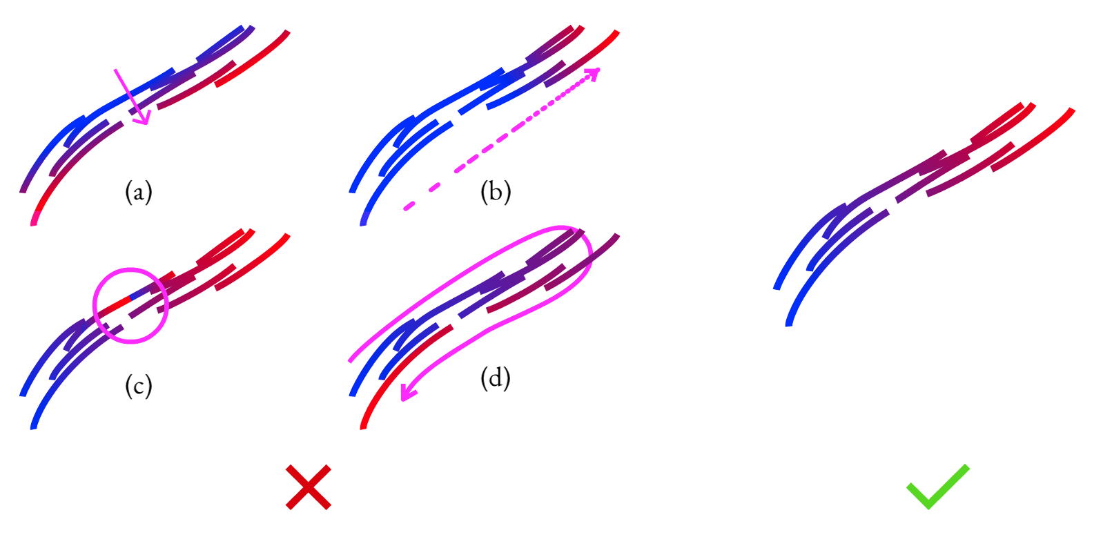
A good parameterization follows stroke tangents (a), preserves the arc length of the strip (b), is monotone along each stroke (c), and has isolines that span all nearby stroke points that are perceived to be adjacent within the strip (d).
Applying this to our formulation from before, we are solving for the parameter value \(u\) at each point on the strip that minimizes an energy function designed to preserve arc length (\(E_\text{length}\)) and keep tangents aligned (\(E_\text{align}\)) while constrained to be monotone along each stroke (the constraint at the end).
Solving
This problem contains both continuous variables (the parameter values \(u\) themselves), and discrete variables (the orientation of each stroke \(o_s\), which is either -1 or 1 to indicate the direction its gradient moves.)
To make this feasible to solve, we first solve for just those discrete stroke orientations to maximize the tangent alignment between nearby strokes. Then, we are free to solve for parameterization with only continuous variables.
We first solve just for the gradient orientations of each stroke in a cluster so that we can subsequently solve for a parameterization with only continuous variables.
Let's take a look at how we get these discrete orientations. If we look just at a pair of strokes at a time, we can decide on a pairwise orientation based on:
- Isoline span, again so that the parameterization at nearby points moves in roughly parallel directions,
- Narrowness, so if we have to choose a side to align a stroke to, we pick the side that gives us narrower strip cross-sections, and
- Tangent compatibility: we want tangents at the same u value to move in roughly the same direction. If we find the tangents would diverge drastically, we prefer an orientation where we flow from one stroke into another without considering them to overlap within the strip.
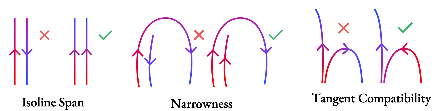
Properties we use to decide on the orientation of a pair of strokes.
Once we've done this for all pairs, we can come up with global orientations by deciding how important each pair's alignment is to the global solution based on its overlap, parallelism, and separation distance. This is a graph labeling problem: we pick stroke orientations that minimize importance-weighted violations of our pairwise orientations.
Once we have our orientations, we can look at the rest of the parameterization formula. We have two energy terms in our parameterization, designed to make the parameterization arc length, and to keep the parameterization gradient aligned with stroke tangents.
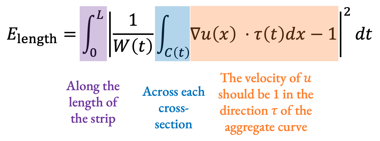
For our arc length preserving term, we integrate along the length of the strip, and across each cross-section, and expect that at each point, u should be changing at a speed of 1 in the direction of the aggregate curve:
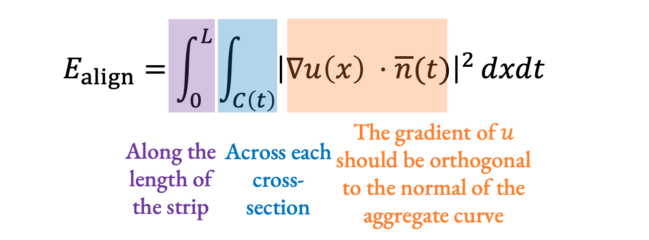
For our tangent alignment term, we again integrate along the length of the strip and across each cross-section, and at each point, we want the gradient of u to be orthogonal to the normal of the aggregate curve. If they are orthogonal everywhere, then the isolines of the parameterization will be orthogonal to the curve, and the tangents will be aligned:
Even with discrete variables removed, this formula is difficult to solve because it's self-referential. The formula refers to the aggregate curve's tangent and normal. We approximate these by averaging stroke tangents on a given cross section. However, the cross sections are the isolines of the parameterization, which is what we're trying to find! So we would need to get that first somehow.
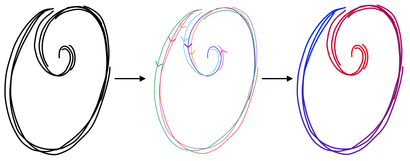
Our solution is to parameterize in three steps:
- First, we use adjacent points to come up with likely cross-sections and parameterize using those, knowing some are outliers.
- Since parameterization tells us the shape of the strip, we can use the parameterization to tell us which of those connections are outliers, and iteratively remove them.
- Then, our parameterization is reliable enough that we can use its isolines of the parameterization at cross-sections, use those to parameterize again to reach a final output.
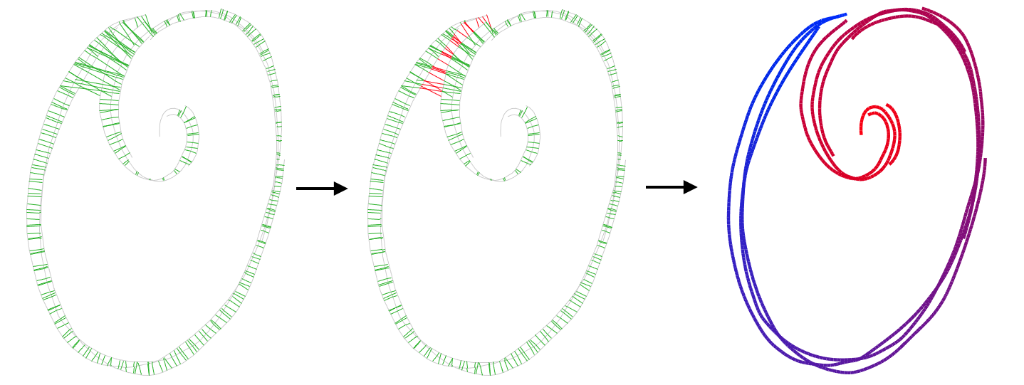
We parameterize by starting with likely-adjacent connections, knowing some are outliers. We parameterize using these to iteratively remove the outliers. Once removed, we can use cross-sections from the previous parameterization to iteratively reach a final parameterization.
We get our initial, likely cross-sections by shooting rays orthogonally from sample points along the input strokes, filtering out big tangent differences and outlier gaps between intersections.
Next, we use a relaxed version of our parameterization designed to figure out which connections are adjacent within the strip. We multiply each connection by a term representing how likely the connection is to be within the strip. Because we know that having different parameter values means two points are on different parts of the strip, this likelihood term is a function of how similar the u values are at each side of a given connection. We alternate between parameterizing based on those likelihoods, and then updating them based on our new u values.
Then, finally, we create new cross-sections from the isolines of the parameterization. We use those new cross-sections to parameterize again, and then repeat this until we converge.
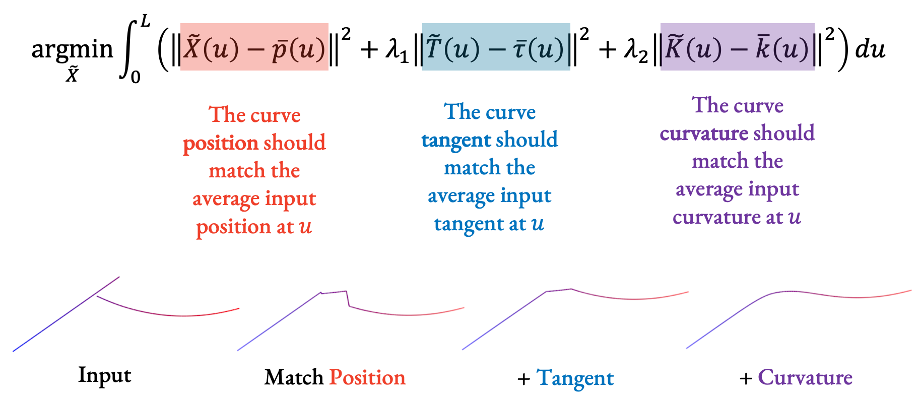
With a parameterization, we can fit a curve! Our goal is to go along each parameter value u and have the fitted curve match the geometric properties of the input strokes at that u value.
When fitting, we care about three properties that we balance:
- The position of the aggregate curve should match the average input position at each u,
- The curve tangent should match the average input tangent, and finally,
- The curvature should also match the average input curvature.
Validation
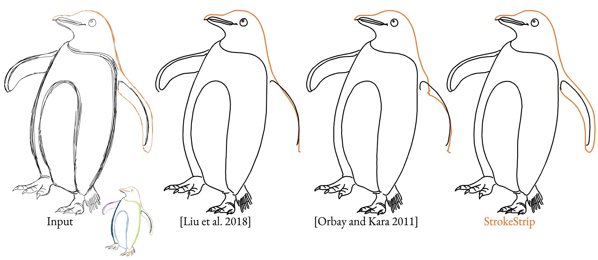
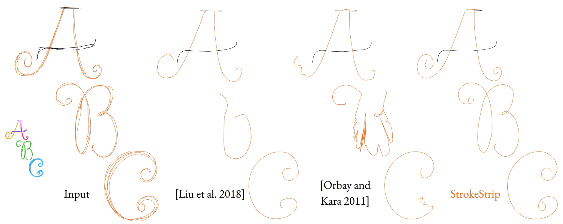
With all of this in place, our method is able to create outputs that match viewer expectations even when given complex inputs, even when prior methods fail.
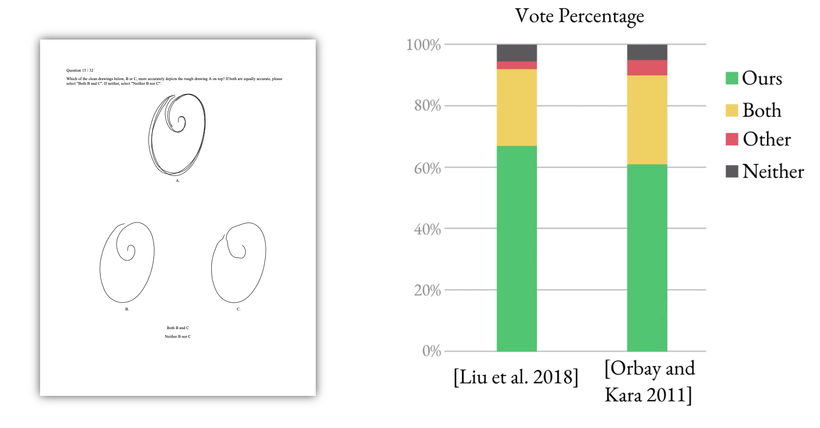
To further validate our method, we ran a user study where we asked viewers to look at an input sketch and decide between which curves from different methods they prefer. We found that our method was preferred by a factor of 12:1 over the next best alternative method.
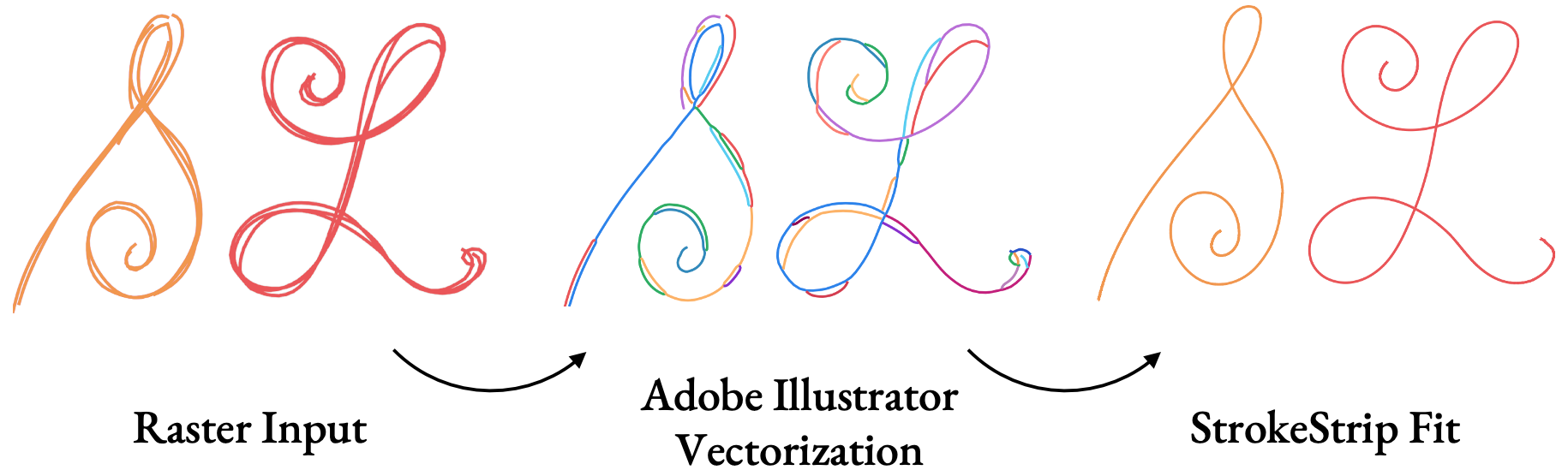
We also tested our method on raster inputs. After running inputs through common vectorization tools, with only minimal changes to the algorithm to account for vectorization artifacts, we produce fitted curves that match expectations.
As mentioned earlier, having a parameterization enables us to edit sketches more easily. Here, we have coloured whole stroke clusters by interpolating colours along each strip.
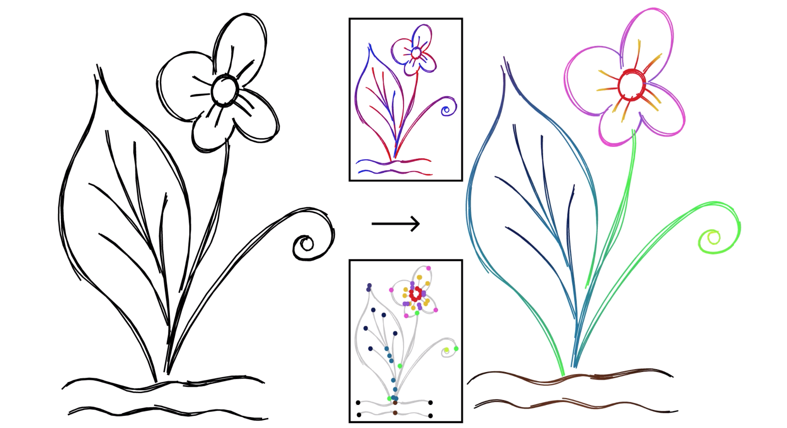
Another benefit of the parameterization and fitting shown here is the ability to edit every stroke in a cluster at once, just using the controls for the cluster’s aggregate curve, instead of having to move around each stroke in the cluster one-by-one.
Conclusion
So, by starting from the arc length parameterization of strips and restricting the domain to input strokes, we open the door to simple parametric fitting and editing that we have shown to be robust across a wide variety of inputs.
You can view our results and supplementary material in more detail on the project website, and view a C++ implementation of the algorithm on GitHub.
Thank you to my co-authors for all of their help making this work happen, to Enrique Rosales, Sari Pagurek van Mossel, and Silver Burla for their drawings, and to Enrique Rosales and Jerry Yin for their additional help on the paper as we got close to the deadline!